
Let’s take a look at the following really useful functions that will help us every day in Excel.
Functions that help with CASE
This set of 3 functions are very handy to use when text has been imported into Excel and it has not arrived in the correct case. Maybe it has gone in with Capital letters and you need lowercase or vice versa.
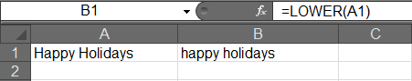
=LOWER()
This will convert the text inside of a cell, so that it all appears in lowercase.

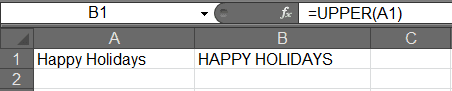
=UPPER()
This will convert the text inside of a cell, so that it all appears in UPPERCASE.

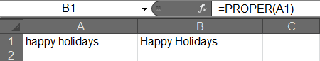
=PROPER()
This will covert the text inside of a cell, so that it all appears with the first letter of each word in UPPERCASE and the rest of the word in lowercase.

Functions that help tidy up
=TRIM()
This formula will get rid, delete, any spaces that may be present at the start or at the end of the contents of a cell. Again this is very useful when data has been imported from a database where the data entered was not accurate enough for Excel and it may have implications when you are doing sorts and filters.
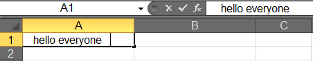
Below we can see a text in cell A1, it has spaces at the start and at the end of the text.
We will use =TRIM() to tidy this up:
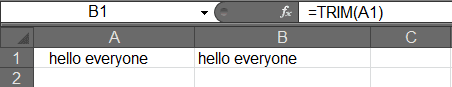
The spaces before and after the contents of cell A1 have been deleted.
Extracting Text
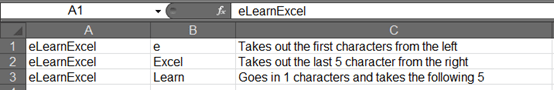
If you would like to extract parts of the contents of a cell, these 3 formulae will help:=LEFT(), =RIGH(), =MID()
Let’s take a look at how these work:
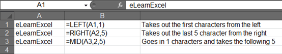
Giving us the following answer:
Functions that will check contents are the same:
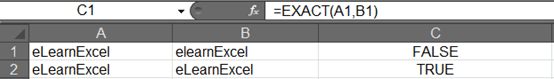
=EXACT()
 This formula will help us to ensure that the contents of 2 cells are identical. This formula is case sensitive and will give you a TRUE or FALSE answer like below:
Functions that will join the content of two cells into one
=CONCATENATE()
Using the “&” symbol
This formula will allow us to take the contents of a number of cells and join them together. Take for exam the following:

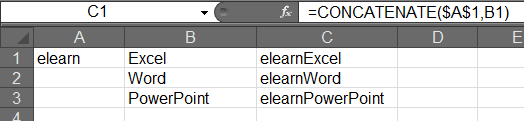
The above formula joins the contents of A1 to the contents of B1 and shows us the join in cell C1. The reason why A1 is absolute (the dollar signs) is because when I drag this formula down it always has to use A1 but the other cell B1 should change to B2, B3 and so on…
If we need to insert a space into the join, for example when joining a title, a first name and a last name, we can use the & symbol instead – it’s actually easier. Let’s take a look:

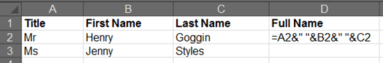
Break it up to understand it.
Below are each of the formula parts – just add a & between them:
A2 = Mr
” ” = a space
B2 = Henry
” ” = a space
C2 = Goggin
Give them a go!